Basic of Probability

Important Definition

1. Random Experiments
   1. An experiment is said to be random if its results cannot be determined beforehand.
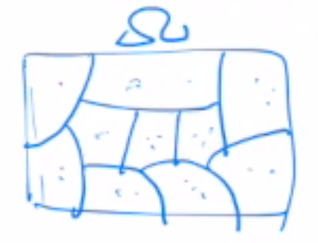
2. Sample Space
   1. The set \(\Omega\) of all possible results of a random experiment is called sample space
   2. A space that contains all possible outcomes / samples
   3. Sample may be numerical or non-numerical
   • Example
     • E: Tossing a coin
       • : \(\Omega = \{H, T\}\)
     • E: Rolling a die
       • : \(\Omega = \{1,2,3,4,5,6\}\)
     • E: # of calls ongoing in telephone exchange
       • : \(\Omega = \{ 0, 1, 2, \cdots, \infty \}\)
     • E: Temperature of a particular city
       • : \(\Omega = \{x \vert 0 < x < 50^o C \}\)
3. The \(\sigma\) field
   1. A collection \(F\) of subsets of \(\Omega\) is called a \(\sigma\) field over \(\Omega\)
      • Condition:
        • (1) \(\Omega \in F\)
        • (2) If \(A \in F\), then \(A^c \in F\), where \(c\) means complement
      • (3) If \(A_1, A_2 , cdots, \in F\), then \(U^\infty_{i=1} A_i \in F\)
      • Example
        • (1) \(\begin{aligned} \Omega &= \{H, T \} \\ F &= \{ \emptyset, \{H\}, \{T\}, \Omega\} \\ F_0 &= \{\emptyset, \Omega\}, \text{which is also called the trivial } \sigma \text{ field} \end{aligned}\)
        • (2) \(\Omega = \{a, b, c\}\)
      • : \(F_0 = \{\emptyset, \Omega\}\)
      • : \(F= \{\emptyset, \{a\}, \{b,c\}, \Omega \}\)
      • : \(F = \{ \emptyset, \{a\}, \{b\} \{c\}, \{a,b\}, \{b,c\}, \{c,a\}, \Omega \}\) - (3) \(\Omega = \mathbb{R} = \{x \vert -\infty < x < \infty \}\)
      • : \(F_0 = \{\emptyset, \Omega\}\)
      • : \(F = \{ \emptyset, \{a\}, (a,b), (a,b], [a,b), [a,b], (-\infty, a),[a, \infty), (a, \infty), \Omega\}\), which is also called Borel \(\sigma\) field on the real line.
4. Probability
   1. Let \(\Omega\) be a sample space
   2. Let \(F\) be a \(\sigma\) field over \(\Omega\)
   3. A real value set function \(P\) defined on \(F\) is called a probabilty if satisfying
      1. \(P(A) \geq 0\) for all \(A \in F\)
      2. \[P(\Omega) = 1\]
      3. If \(A_1, A_2, \cdots\) are mutually disjoint events inf \(F\), then \(P(U_{i=1} A_i) = \sum_i P(A_i)\)
   4. The triplet \((\Omega, F, P)\) is called a probability space
   5. Elements of \(\Omega\) is called sample; Elements of \(\F\) is called events

Review of Probability

Sample space \(\Omega\)

1. a set
2. element of \(\Omega\) : outcomes
3. subset of \(\Omega\) : events

Set theory

1. Set: a collection of distinct element
2. Let \(\Omega: \text{sample space}; A,B \in \Omega\)
3. Union: \(A \cup B = \{x\in \Omega \vert x \in A \text{ or } x \in B \}\)
4. Intersection: \(A \cap B = \{x \in \Omega \verb x \in A \text{ and } x \in B \}\)
5. Complement: \(A^c = \{ x\in \Omega \vert \notin A \}\)
6. Difference: \(A\B = \{ x \in \Omega \vert x\in A \text{ and } x \notin B\}\)

\(\sigma\) field or \(\sigma\) algebra

1. Denote as \(F\), a collection of events
2. : \(F\) represents the set of events for which the probability can be defined
3. \[\Omega \in F\]
4. If \(A \in F\), then\(A^c \in F\)
5. If \(A_1, A_2, ..., \in F\), then \(A_1 \cup A_2 \cup ... \in F\)
6. If (3,4,5) condition fulfilled, then \(F\) is an algebra

Measurable space

• If we get (\(\Omega, F\)) together, we call it as measurable space, as \(F\) contains all the subsets for which we can measure the probability

Probability

• Let us have a measurable space (\(\Omega, F\)), then we define a function \(P_r: F \to [0,1]\), where \(P_r\) is a function to map measurable space to finite number
  1. \[\forall A \in F, 0 \le P_r(A) \le 1\]
  2. \[P_r(\Omega) = 1\]
  3. If \(A, B \in F, A \cap B = \emptyset\), then \(P_r(A \cup B) = P_r(A) + P_r(B)\)
  4. Extend of 3, If \(A_1, A_2, \cdots\) are mutually disjoint events inf \(F\), then \(P(U_{i=1} A_i) = \sum_i P(A_i)\)
  5. If (1,2,3) fulfilled, \(P_r\) is called probability measure

Probability Space

• (\(\Omega, F, P_r\)) is a triplet, formed a probability space

Conditional Probability

• Let say we have events A,B
• then \(P_r(B\vert A) = \frac{P_r(A \cap B)}{P_r(A)}\)
• If \(P_r(B\vert A) = P_r(B)\), then A and B are independent

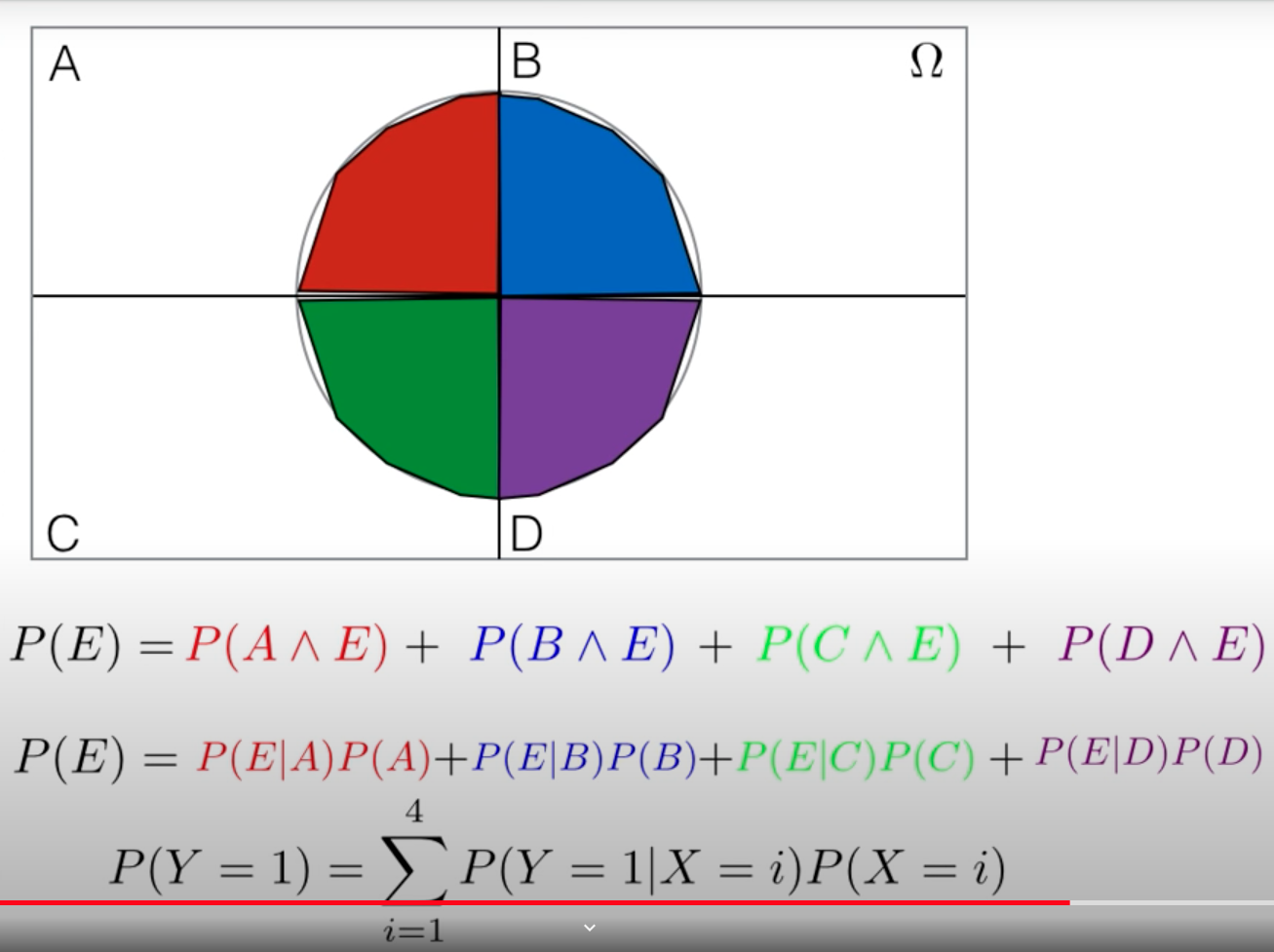
Partition of \(\Omega\)

• We define a sample space to a collection of subsets. They are multually disjoint.
• Let say we have \(\{A_1, A_2, ..., A_k \}\)
  1. The maths expression: \(\cup^R_{i=1}A_i = \Omega\)
  2. \[A_i \cap A_j = \emptyset (i\neq j)\]
  3. Partitiaion Thm (law of total probability)
  • : \(\begin{aligned} P_r(B) &= P_r(\cup^R_{i=1} (B \cap A_i)) \\ &= \sum^R_{i=1} P_r(B \cap A_i), \text{as } A_i \text{ are mutually exhausive} \\ &= \sum^R_{i=1} P_r(B\vert A_i)\cdot P_r(A_i) \end{aligned}\)
  • 

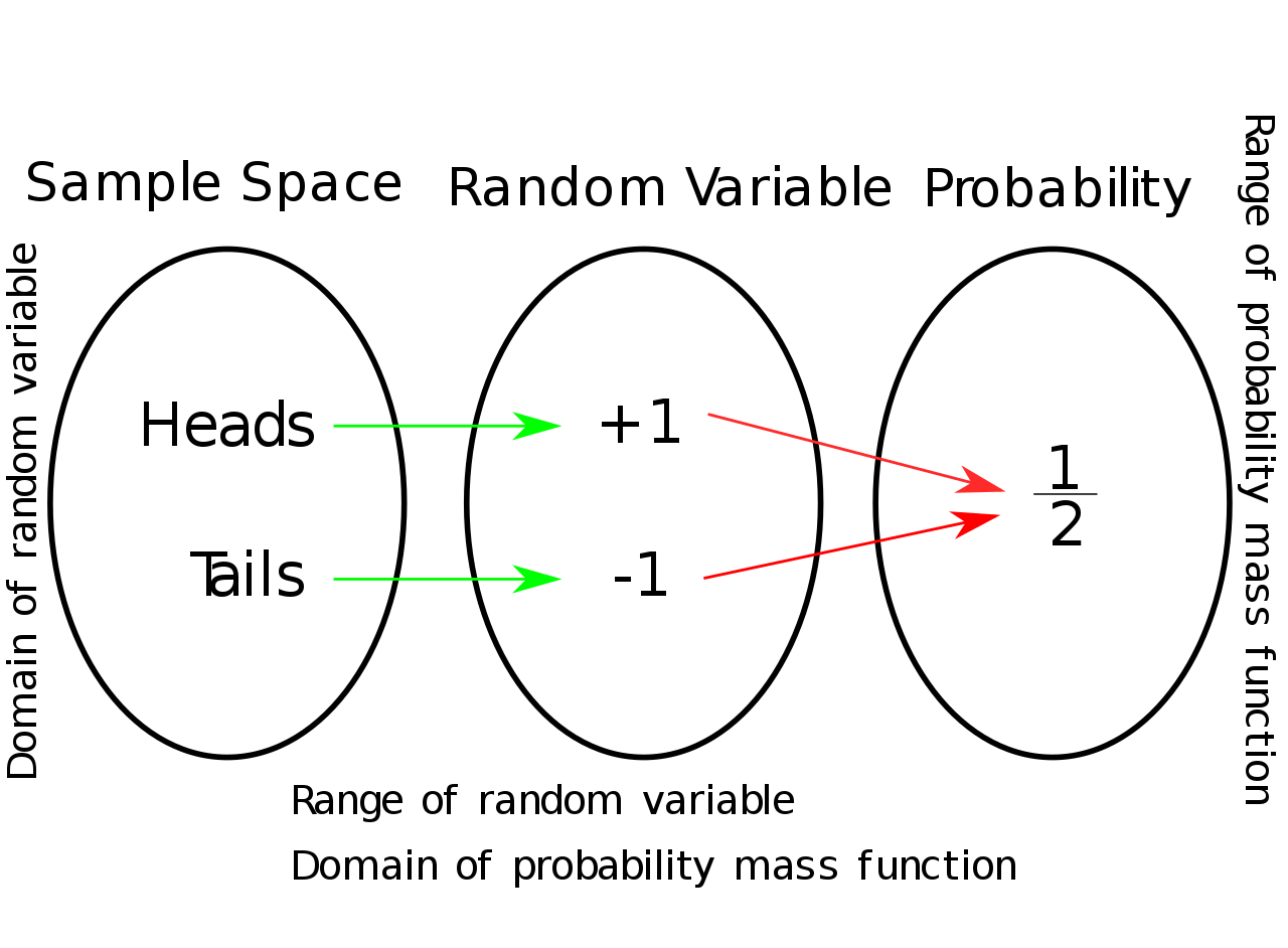
Random variable \(X\)

• Random variable \(X\) is not a variable, it is a function that map \(X:\Omega \to \mathbb{R}\)
• If \(X(\Omega)\) is discrete, then \(X\) is discrete, so for continuous

Shorthand notation \(P_r(X \le x)\)

• :\(X\) is random variable
• :\(x\) is a number
• :\(P_r(X \le x) = P_r(\{\omega \in \Omega \vert X(\omega) \le x\})\)

Probability Mass function

• :\(X\) is discrete
• : \(P(x_i) = P_r(X=x_i) = P_r(\{\omega \in \Omega \vert X(\omega) = x\})\)
• \[) \le P(x_i) \le 1; i=1,2,\cdots\]
• \[\sum^infty_i=1 P(x_i)=1\]
• :\(P_r(X \le x_i) = \sum^R_{i=1}P(x_i)\), also known as cumulative distribution function

Probability Density function

• :\(X\) is continuous
• \[P(X=x) =0\]
• \[P(x_1 < X < x_2) = \int^{x_2}_{x_1} f(x) dx\]
• Property:
  1. : \(f(x) \ge 0\), but \(f(x)\) itself can be greater than 1
  2. Culmulative Density Function (CDF) \(F(x) = P_r(X\le x) = \int^x_-\infty f(x) dx\)

Expected Value (Means)

• Discrete
  • \[\mathbb{E}(x) = \sum_i x_i P_r(x_i)\]
• Continuous
  • \[\int^\infty_{-\infty} xf(x) dx\]
• Both case can we express as
  • \[\mathbb{E}(x) = \int_v x P_r(dx)\]

Variance

• \[Var = \mathbb{E}((X - \mathbb{E}(x))^2) = \int_v (x-\mathbb{E}(x))^2P_r(dx)\]
• \[Var = \begin{cases} \sum_i(x_i-\mathbb{E}(x))^2 P_r(x_i)\\ \int^\infty_{-\infty} (x-\mathbb{E}(x))^2f(x)dx \end{cases}\]

• Previous
  Review: Generative Modeling by Estimating Gradients of the Data Distribution
• Next
  Review: SRDiff: Single Image Super-Resolution with Diffusion Probabilistic Models