Introduction
Yang et.al introduced Generative Modeling by Estimating Gradients of the Data Distribution that can generate high resolution images as diffusion model did.
In the following paragraph, we discuss
- How to approximate Score in image generation
- How to use the Score
Let say we have a dataset with sample $x_1, x_2, \dotsc, x_N$. Each sample $x_i, i \in 1, \dotsc, N$ is drawn from an unknown distribution \(p_{data}(x)\). We want to find out this distribution (hopeful) and make use of this distribution.
We should find the distribution \(p_{data}(x)\) (a closed form). However, it is impossible as \(p_{data}(x)\) is impractical to obtain. By dataset, we can only know the sampling results of \(p_{data}(x)\).
Can we use a score function to replace finding the probability density function p.d.f or probability mass function p.m.f? Yes
A p.d.f should fulfill two things:
- \[p(x) \ge 0 \text{ for all } x \in \mathbb{R}\]
- \[\int^{\infty}_{-\infty} p(x) dx = 1\]
This lead to \(s_\theta(x) = \nabla_x log p_\theta (x)\). Let us forget score function for seconds.
Why \(\nabla_x \log {p(x)}\) ?
Taking log provide a good property, we use log to escape normalization. Consider a p.d.f $q(x)$ which is unnormalized, we should perform an operation s.t. \(p(x) = \frac{e^{-q(x)}}{Z}\), \(Z\) is a normalizing constant to make \(q(x)\) fulfill condition 2.
Second, consider \(\frac{dlog(P)}{dx} = \frac{1}{P}\frac{dP}{dx}\), it is actually calculating the rate of change of function $P$.
Combining two points above, we can have
\[\nabla_{\mathbf{x}} \log p(\mathbf{x})=-\nabla_{\mathbf{x}} p(\mathbf{x})+\underbrace{\nabla_{\mathbf{x}} \log Z}_{=0}=-\nabla_{\mathbf{x}} p(\mathbf{x})\]This score function can
- escape normalization term
- consider the rate of change of captioned distribution
This property is illustrated as gif as well:
Parameterizing probability density functions(pdfs). No matter how you change the model family and parameters, it has to be normalized (area under the curve (AUC) must integrate to one).
Parameterizing score functions. No need to worry about normalization.
Should verify
The gradient should always point to the high density region, making optimization for distribution approximation possible.
Score function $s_\theta(x)$ and score matching
Therefore, we can train a model to approximate the score function
\(s_\theta(x) = \nabla_x log p_\theta (x)\).
We can minimize the Fisher divergence between the model and the data distribution, as (noted that s → S and p → P for visibility):
\[\begin{aligned} L_\theta &= \frac{1}{2}\mathbb{E}\Big( \Vert S_\theta(x) - \nabla_x log P_\theta(x) \Vert^2 \Big) \\ &= \frac{1}{2}\int_{\mathbb{R}^N} P(x) \Vert S_\theta(x) - \nabla_x log P(x) \Vert^2 dx \\ &= \frac{1}{2} \int P(x) \Big( \Vert S_\theta(x) \Vert^2 - 2<S_\theta(x), \nabla_x log P(x)> + \Vert \nabla_x log P(x) \Vert^2 \Big) dx \\ &\sim \int P(x) \Big( \frac{1}{2} \Vert S_\theta(x) \Vert^2 - <S_\theta(x), \nabla_x log P(x) > \Big) dx \\ &= \int P(x) \Big( \frac{1}{2} \Vert S_\theta(x) \Vert^2 + \sum^N_{i=1} \frac{\partial S_\theta^{(i)}(x)}{\partial x_i} \Big) dx \\ \end{aligned}\]Unfortunately, it is still impractical as data distribution is discrete. This leads to MCMC Method and Parzen Method.
For the dot product \(<S_\theta(x), \nabla_x log P(x) >\), we simply it by considering one element $x_i$ in calculation
\(\begin{aligned} &-\int_\mathbb{R}^N S_\theta^{(i)}(x)\frac{\partial}{\partial x_i}logP(x) dx \\ &= -\int_\mathbb{R}^N S_\theta^{(i)}(x)\frac{\partial}{\partial x_i}P(x) dx \\ &= -\Big[ S_\theta^{(i)}(x) \underbrace{P(x)}_{=0} \Big]^{\infty}_{-\infty} + \int^{\infty}_{-\infty} P(x) \frac{\partial}{\partial x_i}S_\theta^{(i)}(x), \text{by integral by part} \end{aligned}\) We take limit as a p.d.f condition 2 define the integral domain $(-\infty, \infty)$ . Remark:
- We add $\frac{1}{2}$ just for simpler calculation when taking integral by part.
- \[\Vert x \Vert^2 = x\cdot x\]
- \[\Vert x + y \Vert^2 = \Vert x \Vert^2 + 2<x, y> + \Vert y \Vert^2\]
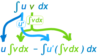
Integral by part
Simple equation as follows: \(\begin{aligned} \int_a^b u(x) v^{\prime}(x) d x & =[u(x) v(x)]_a^b-\int_a^b u^{\prime}(x) v(x) d x \\ & =u(b) v(b)-u(a) v(a)-\int_a^b u^{\prime}(x) v(x) d x . \end{aligned}\)
However, it is not intuitive, it can also be:
Example 1: $\int x cos(x) dx$ \(\begin{aligned} &\int x cos(x) dx \\ &= x sin(x) - \int 1 sin(x) dx \\ &= x sin(x) + cos(x) + Constant \end{aligned}\)
Discrete Case Score Matching
We have \(L_\theta = \int P(x) \Big( \frac{1}{2} \Vert S_\theta(x) \Vert^2 + \sum^N_{i=1} \frac{\partial S_\theta^{(i)}(x)}{\partial x_i} \Big) dx\)
For discrete case, we can use MCMC method to approximate, then we can have
\(\begin{aligned} \tilde{L}_\theta = \frac{1}{2}\sum^n_{t=1}\Big( \frac{1}{2}\Vert S_\theta^{(t)}(x) \Vert^2 + \sum^N_{i=1} \frac{\partial S_\theta^{(i)}(x^{(t)})}{\partial x_i} \Big) \end{aligned}\)
Monte Carlo Markov Chain (MCMC) Method
In the simplist form, for an original expection to be calculated $E_p(f(x))$, we can approximate via MCMC as:
\[\begin{aligned} \mathbb{E}_p(f(x)) &= \int P(x)f(x)dx \\ &\approx \frac{1}{n}\sum^n_{i=1}f(x^{(i)}), \text{ where } x^{(i)} \sim P \end{aligned}\]Continuous Case Score Matching
We understand that $P_{data}(x)$ is basically a p.m.f. However, we want to apply deep learning and back-propagation for much faster calculation than MCMC.
How?
Parzen window (kernel) density estimation
In statistics, kernel density estimation (KDE) is the application of kernel smoothing for probability density estimation, i.e., a non-parametric method to estimate the probability density function of a random variable based on kernels as weights.
Let $(x_1, x_2, \dots, x_n)$ be independent and identically distributed samples drawn from some univariate distribution with an unknown density $ƒ$ at any given point $x$. We are interested in estimating the shape of this function $ƒ$. Its kernel density estimator is
\(f_h(x) = \frac{1}{n} \sum^n_{i=1}K_h(x-x_i)\) where $K$ is the kernel — a non-negative function — and $h > 0$ is a smoothing parameter called the bandwidth. Special case $h=0$ means histogram using step function kernal.
Taking a simplist example with table:
| Sample | 1 | 2 | 3 | 4 | 5 | 6 |
|---|---|---|---|---|---|---|
| Value | -2.1 | -1.3 | -0.4 | 1.9 | 5.1 | 6.2 |
First we draw a histogram, as figure below (LHS). It has right angle and is not differentiable. Now we need to smoothing it by some controllable distribution, usually gaussian kernel. The following example use $\sigma^2 = h =2.5$ as bandwidth.
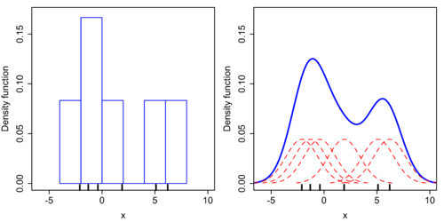
This methods can transfer a p.m.f $P_{data}(x)$ to p.d.f $P_\sigma(x)$ by smoothing techniques
Denoising Score Matching (DSM)
By applying Parzen windows (add noise for smoothing), we have
\[\begin{aligned} L_\theta &= L(\theta)= \frac{1}{2}\int_{\mathbb{R}^N} P(x) \Vert S_\theta(x) - \nabla_x log P(x) \Vert^2 dx \\ L_\sigma(\theta)&= \frac{1}{2}\int_{\mathbb{R}^N} P_\sigma(x) \Vert S_\theta(x) - \nabla_x log P_\sigma(x) \Vert^2 dx \end{aligned}\]However, it is still impractical as we only can input a sample (smoothing by noise) to model and hope the model to find the potential distribution, i.e. we should let pairs of clean and corrupted examples $(x, \tilde{x})$ \(\begin{aligned} x &\sim \{x^{(1)}, \dots, x^{(N)}\} \\ \tilde{x} &\sim P_\sigma(\tilde{x}) \\ P_\sigma(x, \tilde{x}) &= P_{data}(x)P_\sigma(\tilde{x}\vert x) \end{aligned}\)
Therefore, for $L_\sigma(\theta)$, we have
\[\begin{aligned} L^{DSM}_\sigma(\theta) &= \frac{1}{2} \int \int P_\sigma(x, \tilde{x}) \Vert S_\theta (\tilde{x}) - \nabla_{\tilde{x}} log P_\sigma (\tilde{x}\vert x) \Vert^2 d\tilde{x}dx \\ &= \frac{1}{2} \int\int P_{data}(x)P_\sigma(\tilde{x}\vert x)\Vert S_\theta (\tilde{x}) - \nabla_{\tilde{x}} log P_\sigma (\tilde{x}\vert x) \Vert^2 d\tilde{x}dx \\ &=\frac{1}{2} \int P_{data}(x) \int P_\sigma(\tilde{x}\vert x)\Vert S_\theta (\tilde{x}) - \nabla_{\tilde{x}} log P_\sigma (\tilde{x}\vert x) \Vert^2 d\tilde{x}dx \\ \end{aligned}\]For guassian kernal chosen, we have
\[\begin{aligned} P_\sigma(\tilde{x}\vert x) &= \frac{1}{Constant} exp(- \frac{\Vert \tilde{x} - x \Vert^2}{2\sigma^2}) \\ log P_\sigma(\tilde{x}\vert x) &= \tilde{Constant} - \frac{\Vert \tilde{x} - x \Vert^2}{2\sigma^2} \\ \nabla_{\tilde{x}} log P_\sigma(\tilde{x}\vert x) &= - \frac{\tilde{x} - x}{\sigma^2} \end{aligned}\]