Introduction

DDPM maths background and introduction can refer to Review: Denoising Diffusion Probabilistic Models (DDPM)

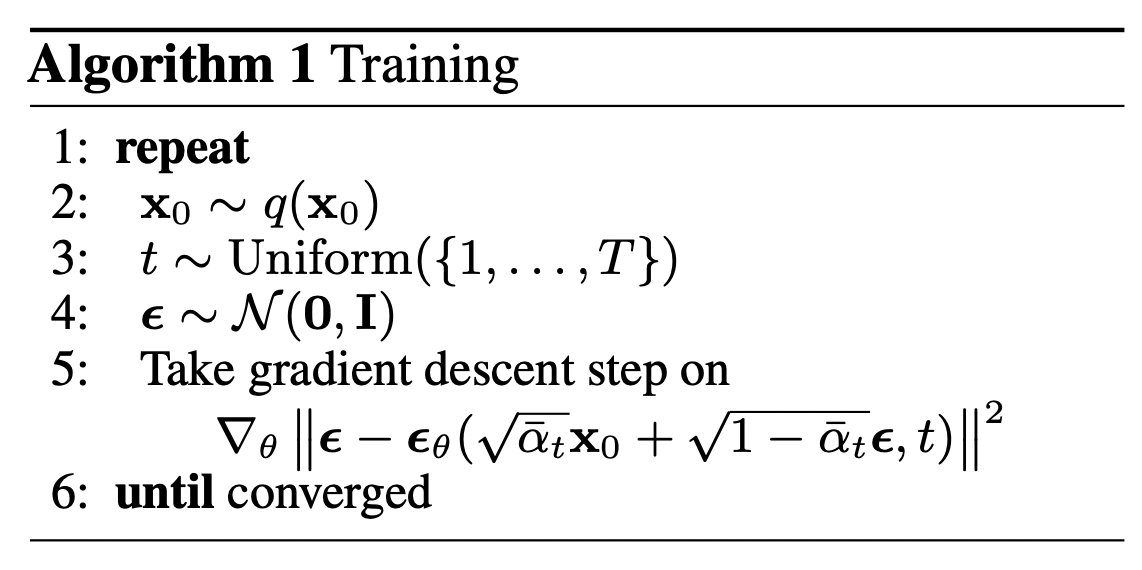
In short, we have a the following training algorithm to be implemented

Model Backbone

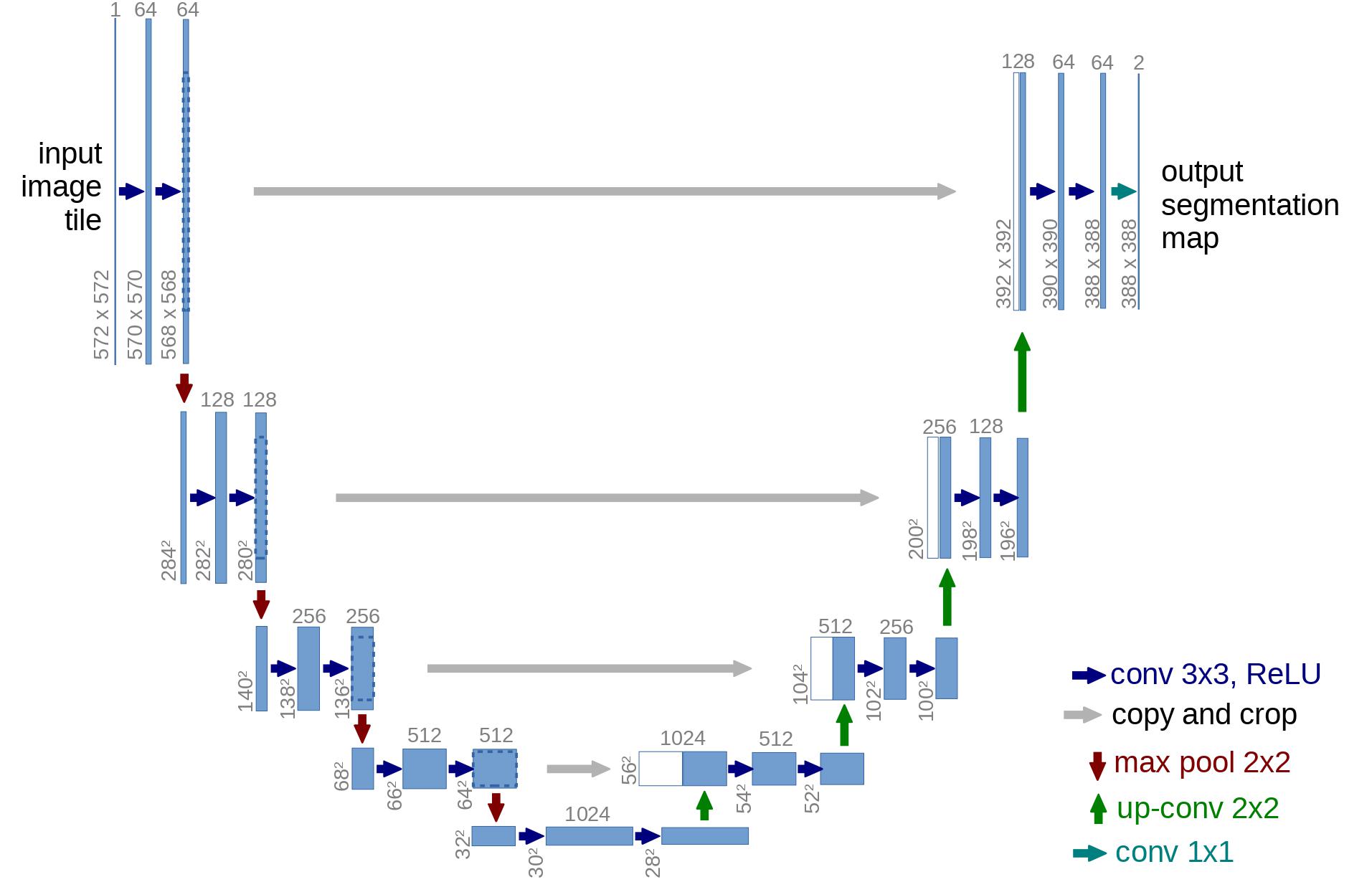
A neural network is applied to implement the reverse process. Technically, the network takes in and outputs tensors of the same shape. Authors has chosen U-Net (Ronneberger et al., 2015) as backbone.

Also, U-Net also introduced residual connections between the encoder and decoder, making a better gradient flow, inspired by ResNet (He et al., 2015).

a U-Net model first downsamples the input (i.e. makes the input smaller in terms of spatial resolution), after which upsampling is performed.

Network Helpers

import math
from inspect import isfunction
from functools import partial

%matplotlib inline
import matplotlib.pyplot as plt
from tqdm.auto import tqdm
from einops import rearrange, reduce
from einops.layers.torch import Rearrange

import torch
from torch import nn, einsum
import torch.nn.functional as F

def exists(x):
    return x is not None

def default(val, d):
    if exists(val):
        return val
    return d() if isfunction(d) else d


def num_to_groups(num, divisor):
    groups = num // divisor
    remainder = num % divisor
    arr = [divisor] * groups
    if remainder > 0:
        arr.append(remainder)
    return arr


class Residual(nn.Module):
    def __init__(self, fn):
        super().__init__()
        self.fn = fn

    def forward(self, x, *args, **kwargs):
        return self.fn(x, *args, **kwargs) + x


def Upsample(dim, dim_out=None):
    return nn.Sequential(
        nn.Upsample(scale_factor=2, mode="nearest"),
        nn.Conv2d(dim, default(dim_out, dim), 3, padding=1),
    )


def Downsample(dim, dim_out=None):
    # No More Strided Convolutions or Pooling
    return nn.Sequential(
        Rearrange("b c (h p1) (w p2) -> b (c p1 p2) h w", p1=2, p2=2),
        nn.Conv2d(dim * 4, default(dim_out, dim), 1),
    )

Positioning Encoding

Inspired by the Transformer (Vaswani et al., 2017), as the parameters of the neural network are shared across time (noise level), the authors employ sinusoidal position embeddings to encode $t$. This makes the neural network “know” at which particular time step (noise level) it is operating, for every image in a batch.

class SinusoidalPositionEmbeddings(nn.Module):
    def __init__(self, dim):
        super().__init__()
        self.dim = dim

    def forward(self, time):
        device = time.device
        half_dim = self.dim // 2
        embeddings = math.log(10000) / (half_dim - 1)
        embeddings = torch.exp(torch.arange(half_dim, device=device) * -embeddings)
        embeddings = time[:, None] * embeddings[None, :]
        embeddings = torch.cat((embeddings.sin(), embeddings.cos()), dim=-1)
        return embeddings

Resnet block

Next, we define the core building block of the U-Net model. The DDPM authors employed a Wide ResNet block (Zagoruyko et al., 2016), but Phil Wang has replaced the standard convolutional layer by a “weight standardized” version, which works better in combination with group normalization (see (Kolesnikov et al., 2019) for details).

class WeightStandardizedConv2d(nn.Conv2d):
    """
    https://arxiv.org/abs/1903.10520
    weight standardization purportedly works synergistically with group normalization
    """

    def forward(self, x):
        eps = 1e-5 if x.dtype == torch.float32 else 1e-3

        weight = self.weight
        mean = reduce(weight, "o ... -> o 1 1 1", "mean")
        var = reduce(weight, "o ... -> o 1 1 1", partial(torch.var, unbiased=False))
        normalized_weight = (weight - mean) * (var + eps).rsqrt()

        return F.conv2d(
            x,
            normalized_weight,
            self.bias,
            self.stride,
            self.padding,
            self.dilation,
            self.groups,
        )


class Block(nn.Module):
    def __init__(self, dim, dim_out, groups=8):
        super().__init__()
        self.proj = WeightStandardizedConv2d(dim, dim_out, 3, padding=1)
        self.norm = nn.GroupNorm(groups, dim_out)
        self.act = nn.SiLU()

    def forward(self, x, scale_shift=None):
        x = self.proj(x)
        x = self.norm(x)

        if exists(scale_shift):
            scale, shift = scale_shift
            x = x * (scale + 1) + shift

        x = self.act(x)
        return x


class ResnetBlock(nn.Module):
    """https://arxiv.org/abs/1512.03385"""

    def __init__(self, dim, dim_out, *, time_emb_dim=None, groups=8):
        super().__init__()
        self.mlp = (
            nn.Sequential(nn.SiLU(), nn.Linear(time_emb_dim, dim_out * 2))
            if exists(time_emb_dim)
            else None
        )

        self.block1 = Block(dim, dim_out, groups=groups)
        self.block2 = Block(dim_out, dim_out, groups=groups)
        self.res_conv = nn.Conv2d(dim, dim_out, 1) if dim != dim_out else nn.Identity()

    def forward(self, x, time_emb=None):
        scale_shift = None
        if exists(self.mlp) and exists(time_emb):
            time_emb = self.mlp(time_emb)
            time_emb = rearrange(time_emb, "b c -> b c 1 1")
            scale_shift = time_emb.chunk(2, dim=1)

        h = self.block1(x, scale_shift=scale_shift)
        h = self.block2(h)
        return h + self.res_conv(x)

Attention

Next, we define the attention module, which the DDPM authors added in between the convolutional blocks. Attention is the building block of the famous Transformer architecture (Vaswani et al., 2017), which has shown great success in various domains of AI, from NLP and vision to protein folding. Phil Wang employs 2 variants of attention: one is regular multi-head self-attention (as used in the Transformer), the other one is a linear attention variant (Shen et al., 2018), whose time- and memory requirements scale linear in the sequence length, as opposed to quadratic for regular attention.

class Attention(nn.Module):
    def __init__(self, dim, heads=4, dim_head=32):
        super().__init__()
        self.scale = dim_head**-0.5
        self.heads = heads
        hidden_dim = dim_head * heads
        self.to_qkv = nn.Conv2d(dim, hidden_dim * 3, 1, bias=False)
        self.to_out = nn.Conv2d(hidden_dim, dim, 1)

    def forward(self, x):
        b, c, h, w = x.shape
        qkv = self.to_qkv(x).chunk(3, dim=1)
        q, k, v = map(
            lambda t: rearrange(t, "b (h c) x y -> b h c (x y)", h=self.heads), qkv
        )
        q = q * self.scale

        sim = einsum("b h d i, b h d j -> b h i j", q, k)
        sim = sim - sim.amax(dim=-1, keepdim=True).detach()
        attn = sim.softmax(dim=-1)

        out = einsum("b h i j, b h d j -> b h i d", attn, v)
        out = rearrange(out, "b h (x y) d -> b (h d) x y", x=h, y=w)
        return self.to_out(out)

class LinearAttention(nn.Module):
    def __init__(self, dim, heads=4, dim_head=32):
        super().__init__()
        self.scale = dim_head**-0.5
        self.heads = heads
        hidden_dim = dim_head * heads
        self.to_qkv = nn.Conv2d(dim, hidden_dim * 3, 1, bias=False)

        self.to_out = nn.Sequential(nn.Conv2d(hidden_dim, dim, 1), 
                                    nn.GroupNorm(1, dim))

    def forward(self, x):
        b, c, h, w = x.shape
        qkv = self.to_qkv(x).chunk(3, dim=1)
        q, k, v = map(
            lambda t: rearrange(t, "b (h c) x y -> b h c (x y)", h=self.heads), qkv
        )

        q = q.softmax(dim=-2)
        k = k.softmax(dim=-1)

        q = q * self.scale
        context = torch.einsum("b h d n, b h e n -> b h d e", k, v)

        out = torch.einsum("b h d e, b h d n -> b h e n", context, q)
        out = rearrange(out, "b h c (x y) -> b (h c) x y", h=self.heads, x=h, y=w)
        return self.to_out(out)

Group Normalization

The DDPM authors interleave the convolutional/attention layers of the U-Net with group normalization.

We define a PreNorm class, which will be used to apply groupnorm before the attention layer, as we’ll see further.

Remark: there’s been a debate about whether to apply normalization before or after attention in Transformers without Tears (Nguyen & Salazar, 2019).

class PreNorm(nn.Module):
    def __init__(self, dim, fn):
        super().__init__()
        self.fn = fn
        self.norm = nn.GroupNorm(1, dim)

    def forward(self, x):
        x = self.norm(x)
        return self.fn(x)

Conditional U-Net

Now that we’ve defined all building blocks (position embeddings, ResNet blocks, attention and group normalization), it’s time to define the entire neural network.

The network takes a batch of noisy images of shape (batch_size, num_channels, height, width) and a batch of noise levels of shape (batch_size, 1) as input, and returns a tensor of shape (batch_size, num_channels, height, width)

Recall the U-Net architecture.

first, a convolutional layer is applied on the batch of noisy images, and position embeddings are computed for the noise levels
next, a sequence of downsampling stages are applied. Each downsampling stage consists of 2 ResNet blocks + groupnorm + attention + residual connection + a downsample operation at the middle of the network, again ResNet blocks are applied, interleaved with attention
next, a sequence of upsampling stages are applied. Each upsampling stage consists of 2 ResNet blocks + groupnorm + attention + residual connection + an upsample operation
finally, a ResNet block followed by a convolutional layer is applied.

class Unet(nn.Module):
    def __init__(
        self,
        dim,
        init_dim=None,
        out_dim=None,
        dim_mults=(1, 2, 4, 8),
        channels=3,
        self_condition=False,
        resnet_block_groups=4,
    ):
        super().__init__()

        # determine dimensions
        self.channels = channels
        self.self_condition = self_condition
        input_channels = channels * (2 if self_condition else 1)

        init_dim = default(init_dim, dim)
        self.init_conv = nn.Conv2d(input_channels, init_dim, 1, padding=0) # changed to 1 and 0 from 7,3

        dims = [init_dim, *map(lambda m: dim * m, dim_mults)]
        in_out = list(zip(dims[:-1], dims[1:]))

        block_klass = partial(ResnetBlock, groups=resnet_block_groups) #partial is used to pre-fill some argument 
        # detail https://www.geeksforgeeks.org/partial-functions-python/

        # time embeddings
        time_dim = dim * 4

        self.time_mlp = nn.Sequential(
            SinusoidalPositionEmbeddings(dim),
            nn.Linear(dim, time_dim),
            nn.GELU(),
            nn.Linear(time_dim, time_dim),
        )

        # layers
        self.downs = nn.ModuleList([])
        self.ups = nn.ModuleList([])
        num_resolutions = len(in_out)

        for ind, (dim_in, dim_out) in enumerate(in_out):
            is_last = ind >= (num_resolutions - 1)

            self.downs.append(
                nn.ModuleList(
                    [
                        block_klass(dim_in, dim_in, time_emb_dim=time_dim),
                        block_klass(dim_in, dim_in, time_emb_dim=time_dim),
                        Residual(PreNorm(dim_in, LinearAttention(dim_in))),
                        Downsample(dim_in, dim_out)
                        if not is_last
                        else nn.Conv2d(dim_in, dim_out, 3, padding=1),
                    ]
                )
            )

        mid_dim = dims[-1]
        self.mid_block1 = block_klass(mid_dim, mid_dim, time_emb_dim=time_dim)
        self.mid_attn = Residual(PreNorm(mid_dim, Attention(mid_dim)))
        self.mid_block2 = block_klass(mid_dim, mid_dim, time_emb_dim=time_dim)

        for ind, (dim_in, dim_out) in enumerate(reversed(in_out)):
            is_last = ind == (len(in_out) - 1)

            self.ups.append(
                nn.ModuleList(
                    [
                        block_klass(dim_out + dim_in, dim_out, time_emb_dim=time_dim),
                        block_klass(dim_out + dim_in, dim_out, time_emb_dim=time_dim),
                        Residual(PreNorm(dim_out, LinearAttention(dim_out))),
                        Upsample(dim_out, dim_in)
                        if not is_last
                        else nn.Conv2d(dim_out, dim_in, 3, padding=1),
                    ]
                )
            )

        self.out_dim = default(out_dim, channels)

        self.final_res_block = block_klass(dim * 2, dim, time_emb_dim=time_dim)
        self.final_conv = nn.Conv2d(dim, self.out_dim, 1)

    def forward(self, x, time, x_self_cond=None):
        if self.self_condition:
            x_self_cond = default(x_self_cond, lambda: torch.zeros_like(x))
            x = torch.cat((x_self_cond, x), dim=1)

        x = self.init_conv(x)
        r = x.clone()

        t = self.time_mlp(time)

        h = []

        for block1, block2, attn, downsample in self.downs:
            x = block1(x, t)
            h.append(x)

            x = block2(x, t)
            x = attn(x)
            h.append(x)

            x = downsample(x)

        x = self.mid_block1(x, t)
        x = self.mid_attn(x)
        x = self.mid_block2(x, t)

        for block1, block2, attn, upsample in self.ups:
            x = torch.cat((x, h.pop()), dim=1)
            x = block1(x, t)

            x = torch.cat((x, h.pop()), dim=1)
            x = block2(x, t)
            x = attn(x)

            x = upsample(x)

        x = torch.cat((x, r), dim=1)

        x = self.final_res_block(x, t)
        return self.final_conv(x)

Defining the forward diffusion process

Schedules

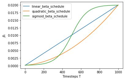
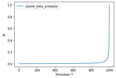
The forward diffusion process gradually adds noise to an image from the real distribution, in a number of time steps $T$. This happens according to a variance schedule. The original DDPM authors employed a linear schedule:

We set the forward process variances to constants increasing linearly from $\beta_1 = 10^{-4} \text{ to } \beta_T = 0.02$

Below, we define various schedules for the $T$ timesteps (we’ll choose one later on).

def cosine_beta_schedule(timesteps, s=0.008):
    """
    cosine schedule as proposed in https://arxiv.org/abs/2102.09672
    """
    steps = timesteps + 1
    x = torch.linspace(0, timesteps, steps)
    alphas_cumprod = torch.cos(((x / timesteps) + s) / (1 + s) * torch.pi * 0.5) ** 2
    alphas_cumprod = alphas_cumprod / alphas_cumprod[0]
    betas = 1 - (alphas_cumprod[1:] / alphas_cumprod[:-1])
    return torch.clip(betas, 0.0001, 0.9999)

def linear_beta_schedule(timesteps):
    beta_start = 0.0001
    beta_end = 0.02
    return torch.linspace(beta_start, beta_end, timesteps)

def quadratic_beta_schedule(timesteps):
    beta_start = 0.0001
    beta_end = 0.02
    return torch.linspace(beta_start**0.5, beta_end**0.5, timesteps) ** 2

def sigmoid_beta_schedule(timesteps):
    beta_start = 0.0001
    beta_end = 0.02
    betas = torch.linspace(-6, 6, timesteps)
    return torch.sigmoid(betas) * (beta_end - beta_start) + beta_start

圖 1
圖 2

To start with, let’s use the linear schedule for $T=300$ time steps and define the various variables from the $\beta_t$ which we will need, such as the cumulative product of the variances $\bar{\alpha}_t$. Each of the variables below are just 1-dimensional tensors, storing values from $t$ to $T$. Importantly, we also define an extract function, which will allow us to extract the appropriate $t$ index for a batch of indices.

timesteps = 300

# define beta schedule
betas = linear_beta_schedule(timesteps=timesteps)

# define alphas 
alphas = 1. - betas
alphas_cumprod = torch.cumprod(alphas, axis=0)
alphas_cumprod_prev = F.pad(alphas_cumprod[:-1], (1, 0), value=1.0)
sqrt_recip_alphas = torch.sqrt(1.0 / alphas)

# calculations for diffusion q(x_t | x_{t-1}) and others
sqrt_alphas_cumprod = torch.sqrt(alphas_cumprod)
sqrt_one_minus_alphas_cumprod = torch.sqrt(1. - alphas_cumprod)

# calculations for posterior q(x_{t-1} | x_t, x_0)
posterior_variance = betas * (1. - alphas_cumprod_prev) / (1. - alphas_cumprod)

alphas_cumprod, alpha_cumprod_prev, sqrt_recip_alphas and posterior_variance

By Pytorch we have a good function to calculate the cumulative product of elements,

Therefore we can calculate $\bar{\alpha_t}$ as:

betas = linear_beta_schedule(timesteps=10)
alphas = 1. - betas
alphas_cumprod = torch.cumprod(alphas, axis=0)
> tensor([0.9999, 0.9976, 0.9931, 0.9864, 0.9776, 0.9667, 0.9537, 0.9389, 0.9222,
        0.9037])

To fix at $\alpha_0 = 1$ s.t. $x_0 = \alpha_0 x_0 + \beta_0\epsilon_0$ to form $\bar{\alpha}_{t-1}$ we need:

alphas_cumprod_prev = F.pad(alphas_cumprod[:-1], (1, 0), value=1.0)
> tensor([1.0000, 0.9999, 0.9976, 0.9931, 0.9864, 0.9776, 0.9667, 0.9537, 0.9389,
        0.9222])

We take recipical for later use

sqrt_recip_alphas = torch.sqrt(1.0 / alphas)
> tensor([1.0000, 1.0012, 1.0023, 1.0034, 1.0045, 1.0056, 1.0068, 1.0079, 1.0090,
        1.0102])

The variance is chosen as $\sigma^2_t = \frac{(1-\bar{\alpha}_{t-1})\beta_t}{1-\bar{\alpha}_t}$

posterior_variance = betas * (1. - alphas_cumprod_prev) / (1. - alphas_cumprod)
> tensor([0.0000e+00, 9.5877e-05, 1.5750e-03, 3.4249e-03, 5.4264e-03, 7.5063e-03,
        9.6330e-03, 1.1791e-02, 1.3971e-02, 1.6168e-02])

Example of forward diffusion process

We’ll illustrate with a cats image how noise is added at each time step of the diffusion process.

from PIL import Image
import requests

url = 'http://images.cocodataset.org/val2017/000000039769.jpg'
image = Image.open(requests.get(url, stream=True).raw)

圖 3

In addition, we need to build an function to transform PIL image with shape 128 dim to tensor $\in [-1,1]$ or vice versa.

from torchvision.transforms import Compose, ToTensor, Lambda, ToPILImage, CenterCrop, Resize

image_size = 128

transform = Compose([
    Resize(image_size),
    CenterCrop(image_size),
    ToTensor(), # turn into Numpy array of shape HWC, divide by 255
    Lambda(lambda t: (t * 2) - 1),
    
])

reverse_transform = Compose([
     Lambda(lambda t: (t + 1) / 2),
     Lambda(lambda t: t.permute(1, 2, 0)), # CHW to HWC
     Lambda(lambda t: t * 255.),
     Lambda(lambda t: t.numpy().astype(np.uint8)),
     ToPILImage(),
])
x_start = transform(image).unsqueeze(0)
x_start = reverse_transform(x_start.squeeze())

圖 4

We can now define the forward diffusion process as in the paper. Importantly, we also define an extract function, which will allow us to extract the appropriate tt index for a batch of indices:

def extract(a, t, x_shape):
    batch_size = t.shape[0]
    out = a.gather(-1, t.cpu())
    return out.reshape(batch_size, *((1,) * (len(x_shape) - 1))).to(t.device)

# forward diffusion (using the nice property)
def q_sample(x_start, t, noise=None):
    if noise is None:
        noise = torch.randn_like(x_start)

    sqrt_alphas_cumprod_t = extract(sqrt_alphas_cumprod, t, x_start.shape)
    sqrt_one_minus_alphas_cumprod_t = extract(
        sqrt_one_minus_alphas_cumprod, t, x_start.shape
    )

    return sqrt_alphas_cumprod_t * x_start + sqrt_one_minus_alphas_cumprod_t * noise

def get_noisy_image(x_start, t):
  # add noise
  x_noisy = q_sample(x_start, t=t)

  # turn back into PIL image
  noisy_image = reverse_transform(x_noisy.squeeze())

  return noisy_image

for t=40, we have get_noisy_image(x_start, t) as

圖 5

Let’s visualize this for various time steps:

import matplotlib.pyplot as plt

# use seed for reproducability
torch.manual_seed(0)

# source: https://pytorch.org/vision/stable/auto_examples/plot_transforms.html#sphx-glr-auto-examples-plot-transforms-py
def plot(imgs, with_orig=False, row_title=None, **imshow_kwargs):
    if not isinstance(imgs[0], list):
        # Make a 2d grid even if there's just 1 row
        imgs = [imgs]

    num_rows = len(imgs)
    num_cols = len(imgs[0]) + with_orig
    fig, axs = plt.subplots(figsize=(200,200), nrows=num_rows, ncols=num_cols, squeeze=False)
    for row_idx, row in enumerate(imgs):
        row = [image] + row if with_orig else row
        for col_idx, img in enumerate(row):
            ax = axs[row_idx, col_idx]
            ax.imshow(np.asarray(img), **imshow_kwargs)
            ax.set(xticklabels=[], yticklabels=[], xticks=[], yticks=[])

    if with_orig:
        axs[0, 0].set(title='Original image')
        axs[0, 0].title.set_size(8)
    if row_title is not None:
        for row_idx in range(num_rows):
            axs[row_idx, 0].set(ylabel=row_title[row_idx])

    plt.tight_layout()

plot([get_noisy_image(x_start, torch.tensor([t])) for t in [0, 50, 100, 150, 199]])

圖 6

Loss function

def p_losses(denoise_model, x_start, t, noise=None, loss_type="l1"):
    if noise is None:
        noise = torch.randn_like(x_start)

    x_noisy = q_sample(x_start=x_start, t=t, noise=noise)
    predicted_noise = denoise_model(x_noisy, t)

    if loss_type == 'l1':
        loss = F.l1_loss(noise, predicted_noise)
    elif loss_type == 'l2':
        loss = F.mse_loss(noise, predicted_noise)
    elif loss_type == "huber":
        loss = F.smooth_l1_loss(noise, predicted_noise)
    else:
        raise NotImplementedError()

    return loss

Datasets Example

Here we use the Datasets library to easily load the Fashion MNIST dataset from the hub (Hugging Face). This dataset consists of images which already have the same resolution, namely 28x28.

from datasets import load_dataset

# load dataset from the hub
dataset = load_dataset("fashion_mnist")
image_size = 28
channels = 1
batch_size = 128

Transform and dataloader as follows:

from torchvision import transforms
from torch.utils.data import DataLoader

# define image transformations (e.g. using torchvision)
transform = Compose([
            transforms.RandomHorizontalFlip(),
            transforms.ToTensor(),
            transforms.Lambda(lambda t: (t * 2) - 1)
])

# define function
def transforms(examples):
   examples["pixel_values"] = [transform(image.convert("L")) for image in examples["image"]]
   del examples["image"]

   return examples

transformed_dataset = dataset.with_transform(transforms).remove_columns("label")

# create dataloader
dataloader = DataLoader(transformed_dataset["train"], batch_size=batch_size, shuffle=True)

Sampling

The sampling algorithm is defined as follows:

圖 8

Generating new images from a diffusion model happens by reversing the diffusion process: we start from $T$, where we sample pure noise from a Gaussian distribution,
and then use our neural network to gradually denoise it (using the conditional probability it has learned), until we end up at time step $t=0$.
As shown above, we can derive a slighly less denoised image $\mathbf{x}_{t-1}$ by plugging in the reparametrization of the mean, using our noise predictor. Remember that the variance is known ahead of time.

@torch.no_grad()
def p_sample(model, x, t, t_index):
    betas_t = extract(betas, t, x.shape)
    sqrt_one_minus_alphas_cumprod_t = extract(
        sqrt_one_minus_alphas_cumprod, t, x.shape
    )
    sqrt_recip_alphas_t = extract(sqrt_recip_alphas, t, x.shape)
    
    # Equation 11 in the paper
    # Use our model (noise predictor) to predict the mean
    model_mean = sqrt_recip_alphas_t * (
        x - betas_t * model(x, t) / sqrt_one_minus_alphas_cumprod_t
    )

    if t_index == 0:
        return model_mean
    else:
        posterior_variance_t = extract(posterior_variance, t, x.shape)
        noise = torch.randn_like(x)
        # Algorithm 2 line 4:
        return model_mean + torch.sqrt(posterior_variance_t) * noise 

# Algorithm 2 (including returning all images)
@torch.no_grad()
def p_sample_loop(model, shape):
    device = next(model.parameters()).device

    b = shape[0]
    # start from pure noise (for each example in the batch)
    img = torch.randn(shape, device=device)
    imgs = []

    for i in tqdm(reversed(range(0, timesteps)), desc='sampling loop time step', total=timesteps):
        img = p_sample(model, img, torch.full((b,), i, device=device, dtype=torch.long), i)
        imgs.append(img.cpu().numpy())
    return imgs

@torch.no_grad()
def sample(model, image_size, batch_size=16, channels=3):
    return p_sample_loop(model, shape=(batch_size, channels, image_size, image_size))

\[\begin{aligned} \text{model means } &= \tilde{\mu}_t = \frac{1}{\sqrt{\alpha_t}}\Big( x_t - \frac{\beta_t }{\sqrt{1-\bar{\alpha}_t}}\epsilon_\theta(x,t) \Big) \\ \text{posterior variance} &= \sigma^2_t = = \frac{(1-\bar{\alpha}_{t-1})\beta_t}{1-\bar{\alpha}_t}\\ \text{return } &= \mathcal{N}(x_{t-1}; \tilde{\mu_t}, \Sigma) x_{t-1} = \tilde{\mu_t} + \sqrt{\sigma^2_t}\epsilon_t \end{aligned}\]

This sampling algorithm is simplifed. More complex implementation, which employs clipping.

Model Training

Next, we train the model in regular PyTorch fashion. We also define some logic to periodically save generated images, using the sample method defined above.

from pathlib import Path

def num_to_groups(num, divisor):
    groups = num // divisor
    remainder = num % divisor
    arr = [divisor] * groups
    if remainder > 0:
        arr.append(remainder)
    return arr

results_folder = Path("./results")
results_folder.mkdir(exist_ok = True)
save_and_sample_every = 1000

We define the model and optimizer from main.

from torch.optim import Adam

device = "cuda" if torch.cuda.is_available() else "cpu"

model = Unet(
    dim=image_size,
    channels=channels,
    dim_mults=(1, 2, 4,)
)
model.to(device)

optimizer = Adam(model.parameters(), lr=1e-3)

Train for 6 epochs

from torchvision.utils import save_image

epochs = 6

for epoch in range(epochs):
    for step, batch in enumerate(dataloader):
      optimizer.zero_grad()

      batch_size = batch["pixel_values"].shape[0]
      batch = batch["pixel_values"].to(device)

      # Algorithm 1 line 3: sample t uniformally for every example in the batch
      t = torch.randint(0, timesteps, (batch_size,), device=device).long()

      loss = p_losses(model, batch, t, loss_type="huber")

      if step % 100 == 0:
        print("Loss:", loss.item())

      loss.backward()
      optimizer.step()

       # save generated images
      if step != 0 and step % save_and_sample_every == 0:
        milestone = step // save_and_sample_every
        batches = num_to_groups(4, batch_size)
        all_images_list = list(map(lambda n: sample(model, batch_size=n, channels=channels), batches))
        all_images = torch.cat(all_images_list, dim=0)
        all_images = (all_images + 1) * 0.5
        save_image(all_images, str(results_folder / f'sample-{milestone}.png'), nrow = 6)

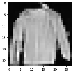
Inference

To sample from the model, we can just use our sample function defined above:

# sample 64 images
samples = sample(model, image_size=image_size, batch_size=64, channels=channels)

# show a random one
random_index = 5
plt.imshow(samples[-1][random_index].reshape(image_size, image_size, channels), cmap="gray")

圖 9

GIF for denoising process

import matplotlib.animation as animation

random_index = 53

fig = plt.figure()
ims = []
for i in range(timesteps):
    im = plt.imshow(samples[i][random_index].reshape(image_size, image_size, channels), cmap="gray", animated=True)
    ims.append([im])

animate = animation.ArtistAnimation(fig, ims, interval=50, blit=True, repeat_delay=1000)
animate.save('diffusion.gif')
plt.show()

Code Review: Denoising Diffusion Probabilistic Models (DDPM)