Denoising Diffusion Implicit Models (DDIM)

Song et. al. (2021) introduced Denoising Diffusion Implicit Models. The concept of DDIM is to apply a new sampling method s.t. the denoising process can be speed up by given a closed form for reverse process.

Recall for DDPM Bayes Derivation

\[\begin{aligned}p(\boldsymbol{x}_t|\boldsymbol{x}_{t-1})\xrightarrow{\text{derive}}p(\boldsymbol{x}_t|\boldsymbol{x}_0)\xrightarrow{\text{derive}}p(\boldsymbol{x}_{t-1}|\boldsymbol{x}_t, \boldsymbol{x}_0)\xrightarrow{\text{approx}}p(\boldsymbol{x}_{t-1}|\boldsymbol{x}_t)\end{aligned}\]
We have found that

Loss function is only related to $p(x_t\vert x_0)$

Sampling process only rely on $p(x_{t-1} \vert x_t)$, where the reverse process is a markov chain

Therefore, we can make a further assumption based on the derivation result. Can we skip $p(x_t\vert x_{t-1})$ during the derivation process s.t.

\[p(\boldsymbol{x}_t|\boldsymbol{x}_{t-1})\xrightarrow{\text{derive}}p(\boldsymbol{x}_t|\boldsymbol{x}_0)\xrightarrow{\text{derive}}p(\boldsymbol{x}_{t-1}|\boldsymbol{x}_t, \boldsymbol{x}_0)\]

DDIM Proof

Mathematical Induction

Mathematical induction is a method for proving that a statement $P(n)$ is true for every natural number n, that is, that the infinitely many cases $P(0), P(1), P(2), P(3), \dots$ all hold.

The following steps should be followed.

$P(1)$ is true
$P(k)$ is true, implying $P(k+1)$ is true
Then $P(n)$ is true for all $n \in \mathbb{N}$

Assumption

Song et. al. (2021) introduced a new equation in DDIM. $q_\sigma\left(\boldsymbol{x}_{t-1} \mid \boldsymbol{x}_t, \boldsymbol{x}_0\right)=\mathcal{N}\left(\sqrt{\alpha_{t-1}} \boldsymbol{x}_0+\sqrt{1-\alpha_{t-1}-\sigma_t^2} \cdot \frac{\boldsymbol{x}_t-\sqrt{\alpha_t} \boldsymbol{x}_0}{\sqrt{1-\alpha_t}}, \sigma_t^2 \boldsymbol{I}\right)$

where all $\alpha$ is equal to $\bar{\alpha}$ in DDPM.

and

$q_\sigma\left(\boldsymbol{x}_t \mid \boldsymbol{x}_0\right)=\mathcal{N}\left(\sqrt{\alpha_t} \boldsymbol{x}_0,\left(1-\alpha_t\right) \boldsymbol{I}\right)$, which is proven in DDPM.

Proof by Mathematical Induction

The statement is as follows:

Assume for any $t \leq T, q_\sigma\left(\boldsymbol{x}_t \mid \boldsymbol{x}_0\right)=\mathcal{N}\left(\sqrt{\alpha_t} \boldsymbol{x}_0,\left(1-\alpha_t\right) \boldsymbol{I}\right)$ holds, if $q_\sigma\left(\boldsymbol{x}_{t-1} \mid \boldsymbol{x}_0\right)=\mathcal{N}\left(\sqrt{\alpha_{t-1}} \boldsymbol{x}_0,\left(1-\alpha_{t-1}\right) \boldsymbol{I}\right)$ , then we can prove the statment by MI for $t$ from $T$ to $1$.

Following the first step of MI, now we need to combine two equation above to calculate $q\sigma(\boldsymbol{x}_{t-1}\vert \boldsymbol{x}_0)$ by law of total probability

\[q_\sigma\left(\boldsymbol{x}_{t-1} \mid \boldsymbol{x}_0\right):=\int_{\boldsymbol{x}_t} q_\sigma\left(\boldsymbol{x}_t \mid \boldsymbol{x}_0\right) q_\sigma\left(\boldsymbol{x}_{t-1} \mid \boldsymbol{x}_t, \boldsymbol{x}_0\right) \mathrm{d} \boldsymbol{x}_t\]

where $q_\sigma\left(\boldsymbol{x}_{t-1} \mid \boldsymbol{x}_0\right)=\mathcal{N}\left(\sqrt{\alpha_{t-1}} \boldsymbol{x}_0,\left(1-\alpha_{t-1}\right) \boldsymbol{I}\right)$ in DDPM.

Finding $\mu_{t-1}$

First, we need to find out $\mu_{t-1}$

\[\begin{aligned} \mu_{t-1} &= \mathbb{E}[x_{t-1}\vert x_0] = \mathbb{E}_{x_t \vert x_0}\big[\mathbb{E}[x_{t-1}\vert x_t, x_0]\big] \\ &= \mathbb{E}_{x_t \vert x_0}[\sqrt{\alpha_{t-1}}x_0 + \sqrt{1-\alpha_{t-1}-\sigma^2_t}\frac{x_t-\sqrt{\alpha_t}x_0}{\sqrt{1-\alpha_t}}] \\ &= \sqrt{\alpha_{t-1}}x_0 + \sqrt{1-\alpha_{t-1}-\sigma^2_t}\frac{\mathbb{E}[x_t\vert x_0]-\sqrt{\alpha_t}x_0}{\sqrt{1-\alpha_t}}, \text{ as conditional to } x_0 \\ &= \sqrt{\alpha_{t-1}}x_0 + \sqrt{1-\alpha_{t-1}-\sigma^2_t}\frac{\sqrt{\alpha_t}x_0-\sqrt{\alpha_t}x_0}{\sqrt{1-\alpha_t}} \\ &= \sqrt{\alpha_{t-1}}x_0 \end{aligned}\]

Finding $\Sigma_{t-1}$

Before finding $\Sigma_{t-1}$, we need to apply Conditional Variance.

Proof for Law of Total Variance

$\begin{aligned} Var(X\vert Y) &:= E[(X-E[X\vert Y])^2 \vert Y] \\ Var(Y) &= E(Y^2) - E(Y)^2 \\ E(Y^2) &= Var(Y) + E(Y)^2 \\ &= E[Var(Y\vert X) + E(Y\vert X)^2], \text{ by law of total expectation} \\ E(Y^2) - E(Y)^2 &= E[Var(Y\vert X) + E(Y\vert X)^2] - E(Y)^2 \\ &= E[Var(Y\vert X) + E(Y\vert X)^2] - E[E(Y \vert X)]^2, \text{ by law of total expectation} \\ &= E[Var(Y\vert X)] + \Big(E[E(Y\vert X)^2] - E[E(Y \vert X)]^2 \Big) \\ \therefore Var(Y) &= E[Var(Y\vert X)] + Var(E[Y\vert X]) \end{aligned}$

where Law of Total Expectation is proven here.

The proof above is also true in vector version.

Proof

From $q_\sigma\left(\boldsymbol{x}_{t-1} \mid \boldsymbol{x}_t, \boldsymbol{x}_0\right)=\mathcal{N}\left(\sqrt{\alpha_{t-1}} \boldsymbol{x}_0+\sqrt{1-\alpha_{t-1}-\sigma_t^2} \cdot \frac{\boldsymbol{x}_t-\sqrt{\alpha_t} \boldsymbol{x}_0}{\sqrt{1-\alpha_t}}, \sigma_t^2 \boldsymbol{I}\right)$ , we can have $Var(x_{t-1} \vert x_t, x_0) = \sigma^2_t \boldsymbol{I}$ and $\mathbb{E}[x_{t-1} \vert x_t, x_0] = \sqrt{1-\alpha_{t-1}-\sigma_t^2} \cdot \frac{\boldsymbol{x}_t}{\sqrt{1-\alpha_t}} + \text{ sth related to } x_0$

\[\begin{aligned} \therefore Var(\mathbb{E}[x_{t-1} \vert x_t, x_0]) &= \frac{1-\alpha_{t-1} - \sigma^2_t}{1 - \alpha_t} Var(x_t \vert x_0) \\ &=\frac{1-\alpha_{t-1} - \sigma^2_t}{1 - \alpha_t}(1-\alpha_t)\boldsymbol{I} \\ &= (1-\alpha_{t-1} - \sigma^2_t)\boldsymbol{I} \\ \therefore \Sigma_{t-1} &= Var(x_{t-1}) = E[Var( x_{t-1}\vert x_t, x_0)] + Var(E[x_{t-1}\vert x_t, x_0]) \\ &= \mathbb{E}[\sigma^2_t\boldsymbol{I}] + (1-\alpha_{t-1} - \sigma^2_t)\boldsymbol{I} = (1-\alpha_{t-1})\boldsymbol{I} \end{aligned}\]

This suggests $q_\sigma\left(\boldsymbol{x}_{t-1} \mid \boldsymbol{x}_t, \boldsymbol{x}_0\right)=\mathcal{N}\left(\sqrt{\alpha_{t-1}} \boldsymbol{x}_0+\sqrt{1-\alpha_{t-1}-\sigma_t^2} \cdot \frac{\boldsymbol{x}_t-\sqrt{\alpha_t} \boldsymbol{x}_0}{\sqrt{1-\alpha_t}}, \sigma_t^2 \boldsymbol{I}\right)$ is true for $t$ from $T$ to $1$.

More useful closed form for sampling

we can derive a more useful closed form s.t.

\[\begin{aligned} q_\sigma\left(\boldsymbol{x}_{t-1} \mid \boldsymbol{x}_t, \boldsymbol{x}_0\right)&=\mathcal{N}\left(\sqrt{\alpha_{t-1}} \boldsymbol{x}_0+\sqrt{1-\alpha_{t-1}-\sigma_t^2} \cdot \frac{\boldsymbol{x}_t-\sqrt{\alpha_t} \boldsymbol{x}_0}{\sqrt{1-\alpha_t}}, \sigma_t^2 \boldsymbol{I}\right) \\ x_t &= \sqrt{\alpha_t}x_0 + \sqrt{1-\alpha_t}\epsilon^{(t)}_\theta(x_t) \\ \therefore x_{t-1} &:= \sqrt{\alpha_{t-1}} \boldsymbol{x}_0+\sqrt{1-\alpha_{t-1}-\sigma_t^2} \cdot \frac{\boldsymbol{x}_t-\sqrt{\alpha_t} \boldsymbol{x}_0}{\sqrt{1-\alpha_t}} + \sigma_t \epsilon_t \\ &= \sqrt{\alpha_{t-1}} \underbrace{\left(\frac{\boldsymbol{x}_t-\sqrt{1-\alpha_t} \epsilon_\theta^{(t)}\left(\boldsymbol{x}_t\right)}{\sqrt{\alpha_t}}\right)}_{\text {"predicted } \boldsymbol{x}_0 \text { " }} +\underbrace{\sqrt{1-\alpha_{t-1}-\sigma_t^2} \cdot \epsilon_\theta^{(t)}\left(\boldsymbol{x}_t\right)}_{\text {“direction pointing to } \boldsymbol{x}_t \text {"}}+\underbrace{\sigma_t \epsilon_t}_{\text {random noise }} \end{aligned}\]

Freedom on Variance $\sigma^2_t$

We can observe that we have a new hyperparameter $\sigma^2_t$. We can take some example from previous blog.

1. Take $\sigma^2_t=\frac{(1-\bar{\alpha}_{t-1})\beta_t}{(1-\bar{\alpha_t})}$ (Same as DDPM)

The paper in DDIM has discussed the performance when $\sigma^2_t= \eta\frac{(1-\bar{\alpha}_{t-1})\beta_t}{(1-\bar{\alpha_t})}, \eta \in [0,1]$

2. Take $\sigma^2_t=0$

By letting $\sigma^2_t=0$ and starting at $x_\tau=z$ , the reversed pass process will become deterministic, meaning that model will generate predicted $x_0$ directly.

Speed up from Non-Markov Inference Pass

圖 1
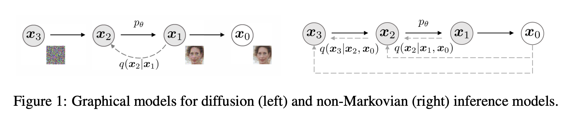
We can observe that we skipped $p(x_t\vert x_{t-1})$ . $\alpha_t$ and $\bar{\alpha}_t$ is deterministic and are hyperparameters. As denoising objective $\left\Vert\boldsymbol{\varepsilon} - \boldsymbol{\epsilon}_{\boldsymbol{\theta}}(\bar{\alpha}_t \boldsymbol{x}_0 + \bar{\beta}_t \boldsymbol{\varepsilon}, t)\right\Vert^2$ (which describe we want a model to predict $x_0$ from $x_t$) does not depend on the specific forward procedure as long as $p(x_t|x_0)$ is fixed, we may also consider forward processes with lengths smaller than T, which accelerates the corresponding generative processes without having to train a different model.

In DDIM view, if we have trained $x_1, x_2, \dots, x_{1000}$ to predict $x_0$, meaning we have 1000 model that train to map $x_1 \rightarrow x_0, x_2 \rightarrow x_0, \dots, x_{1000} \rightarrow x_0$.

圖 2

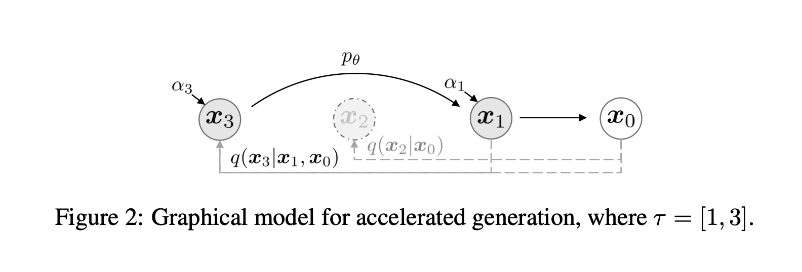
More specifically, we let $\mathbf{\tau} = [\tau_1, \tau_2, \dots, \tau_{dim(\tau)}]$ as an arbitary subset of $[1,2,\dots,T]$ of length $S$. For a well-pretrained diffusion model, the model include the result for any arbitary subset $\mathbf{\tau}$.

Vice versa, we can treat a DDPM with $T$ step is a superset of $\mathbf{\tau}$. If so, we can generate a new image with only $dim(\tau)$ steps.

But dont we train a model with only $dim(\tau)$ step?

In principle, this means that we can train a model with an arbitrary number of forward steps but only sample from some of them in the generative process.

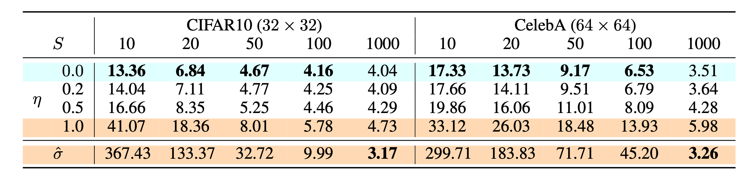
Performance in Different Distribution

The paper in DDIM has discussed the performance in different setting of $\eta$ and $S$, where $S$ means timestep and $\eta$ is a hyperparameter to scale the randomness.

$\sigma^2_t= \eta\frac{(1-\bar{\alpha}_{t-1})\beta_t}{(1-\bar{\alpha_t})}, \eta \in [0,1]$ In experiment, both DDPM($\eta=1$) and DDIM($\eta=0$) is trained with T=1000. They observed that DDIM can produce the best quality samples when $S=dim(\tau)$ is small while DDPM does perform better when we can afford to run the full reverse Markov diffusion steps $(S=T=1000)$.

(Old) The Methods of Undetermined Coefficient

In short, it is just like let $ax^2+bx+c=0$ …

Recall that we have found $\begin{align} p(x_{t-1}\vert x_t, x_0) &= \mathbb{N}(x_{t-1}; \mu(x_{t-1}\vert x_t, x_0), \Sigma(x_{t-1}\vert x_t, x_0)) \nonumber \\ &= \mathbb{N}(x_{t-1}; (\sqrt{\bar{\alpha}_{t-1}} - \frac{\alpha_t(1-\bar{\alpha}_{t-1})}{1-\bar{\alpha}_{t}}) x_{0} + \frac{\sqrt{\alpha_t}(1-\bar{\alpha}_{t-1})}{1-\bar{\alpha}_{t}} x_t, \frac{(1-\bar{\alpha}_{t-1})\beta_t}{(1-\bar{\alpha_t})}I) \end{align}$ We just need the model to fulfill marginal probability s.t.

\[\int p(x_{t-1}\vert x_t,x_0)p(x_t\vert x_0)d x_t = p(x_{t-1}\vert x_0)\]

Therefore, this time we can more generally let

\[\begin{equation} p(\boldsymbol{x}_{t-1}|\boldsymbol{x}_t, \boldsymbol{x}_0) = \mathcal{N}(\boldsymbol{x}_{t-1}; \kappa_t \boldsymbol{x}_t + \lambda_t \boldsymbol{x}_0, \sigma_t^2 \boldsymbol{I}) \end{equation}\]

and form a table as follows: \(\begin{array}{c|c|c} \hline \text{Notation} & \text{Meaning} & \text{Sampling}\\ \hline p(\boldsymbol{x}_{t-1}|\boldsymbol{x}_0) & \mathcal{N}(\boldsymbol{x}_{t-1};\sqrt{\bar{\alpha}_{t-1}} \boldsymbol{x}_0,(1-\bar{\alpha}_{t-1}) \boldsymbol{I}) & \boldsymbol{x}_{t-1} = \sqrt{\bar{\alpha}_{t-1}} \boldsymbol{x}_0 + \sqrt{(1-\bar{\alpha}_{t-1})} \boldsymbol{\varepsilon} \\ \hline p(\boldsymbol{x}_t|\boldsymbol{x}_0) & \mathcal{N}(\boldsymbol{x}_t;\sqrt{\bar{\alpha}_t}\boldsymbol{x}_0,(1-\bar{\alpha}_t) \boldsymbol{I}) & \boldsymbol{x}_t = \sqrt{\bar{\alpha}_t} \boldsymbol{x}_0 + \sqrt{(1-\bar{\alpha}_t)} \boldsymbol{\varepsilon}_1 \\ \hline p(\boldsymbol{x}_{t-1}|\boldsymbol{x}_t, \boldsymbol{x}_0) & \mathcal{N}(\boldsymbol{x}_{t-1}; \kappa_t \boldsymbol{x}_t + \lambda_t \boldsymbol{x}_0, \sigma_t^2 \boldsymbol{I}) & \boldsymbol{x}_{t-1} = \kappa_t \boldsymbol{x}_t + \lambda_t \boldsymbol{x}_0 + \sigma_t \boldsymbol{\varepsilon}_2 \\ \hline {\begin{array}{c}\int p(\boldsymbol{x}_{t-1}|\boldsymbol{x}_t, \boldsymbol{x}_0) \\ p(\boldsymbol{x}_t|\boldsymbol{x}_0) d\boldsymbol{x}_t\end{array}} = p(x_{t-1}\vert x_0) & & {\begin{aligned}\boldsymbol{x}_{t-1} =&\, \kappa_t \boldsymbol{x}_t + \lambda_t \boldsymbol{x}_0 + \sigma_t \boldsymbol{\varepsilon}_2 \\ =&\, \kappa_t (\sqrt{\bar{\alpha}_t} \boldsymbol{x}_0 + \sqrt{(1-\bar{\alpha}_t)} \boldsymbol{\varepsilon}_1) + \lambda_t \boldsymbol{x}_0 + \sigma_t \boldsymbol{\varepsilon}_2 \\ =&\, (\kappa_t \sqrt{\bar{\alpha}_t} + \lambda_t) \boldsymbol{x}_0 + (\kappa_t\sqrt{ (1-\bar{\alpha}_t)} \boldsymbol{\varepsilon}_1 + \sigma_t \boldsymbol{\varepsilon}_2) \\ =& (\kappa_t \sqrt{\bar{\alpha}_t} + \lambda_t) \boldsymbol{x}_0 + \sqrt{\kappa_t^2(1-\bar{\alpha}_t) + \sigma_t^2} \boldsymbol{\varepsilon} \\ \end{aligned}} \\ \hline \end{array}\)

Therefore, we just have 2 equation for 3 unknown, let a free parameter $\sigma^2$ and define:

\[\begin{cases} \sqrt{\bar{\alpha}_{t-1}} &= (\kappa_t \sqrt{\bar{\alpha}_t} + \lambda_t) \\ 1 - \bar{\alpha}_{t-1} &= \sqrt{\kappa_t^2(1-\bar{\alpha}_t) + \sigma_t^2} \\ \end{cases} \\ \begin{align} \kappa_t = \sqrt{\frac{(1-\bar{\alpha}_{t-1})^2 - \sigma_t^2}{1-\bar{\alpha}_t}},\qquad \lambda_t = \sqrt{\bar{\alpha}_{t-1}} - \sqrt{\bar{\alpha}_t}\sqrt{\frac{(1-\bar{\alpha}_{t-1})^2 - \sigma_t^2}{1-\bar{\alpha}_t}} \\ \therefore p_\sigma\left(\mathbf{x}_{t-1} \mid \mathbf{x}_t, \mathbf{x}_0\right)=\mathcal{N}\left(\mathbf{x}_{t-1} ; \sqrt{\alpha_{t-1}} \mathbf{x}_0+\sqrt{1-\alpha_{t-1}-\sigma_t^2} \frac{\mathbf{x}_t-\sqrt{\alpha_t} \mathbf{x}_0}{\sqrt{1-\alpha_t}}, \sigma_t^2 \mathbf{I}\right) \end{align}\]

Review: Denoising Diffusion Implicit Models (DDIM)